Simulation of k-multipole emission patterns
In this tutorial, an electric octupole transition (E3) of a vastly simplified atom, consisting of only two magnetic substates, is excited and the photon scattering rate is calculated for all emission angles.
import matplotlib.pyplot as plt
import numpy as np

import qspec as qs
import qspec.simulate as sim

f_eg = 7e8  # Transition frequency
a_eg = 10.  # Einstein coefficient

g_hyper = [0.]  # HFS A-constant of the g state
e_hyper = [5.]  # HFS A-constant of the e state

i, jg, je = 0., 2., 5.
dm = 1  # The change of the m quantum number

g = sim.State(0., parity="e", j=jg, i=i, f=jg + i, m=jg + i,
              hyper_const=g_hyper, label="g")
e = sim.State(f_eg, parity="o", j=je, i=i, f=je + i, m=jg + i + dm,
              hyper_const=e_hyper, label="e")

states = [g, e]
decay = sim.DecayMap(labels=[("g", "e")], a=[a_eg], k_max=int(je - jg))
atom = sim.Atom(states=states, decay_map=decay)
print(atom.get_multipole_types("g", "e"))
# >>> {'e3'}

intensity = 1e3
pol_eg = sim.Polarization([1., 0, 1j], vec_as_q=False)
laser_eg = sim.Laser(freq=f_eg, polarization=pol_eg,
                     intensity=intensity, k=[0., 1., 0.])

B = [0., 0., 1e-6]  # The B-field vector
env = sim.Environment(B=B)
inter = sim.Interaction(atom=atom, lasers=[laser_eg, ],
                        environment=env, delta_max=1000.)

t = np.linspace(0., 1., 301)  # Create an array of times to simulate
y0 = qs.unit_vector(0, 2, dtype=float)  # Create initial population [1., 0.]

rho = inter.master(t, y0=y0)
y = sim.density_matrix_diagonal(rho, axis=1)[0]

plt.figure(figsize=(6, 4))
plt.plot(t, y[0], label=g.label)
plt.plot(t, y[1], label=e.label)
plt.legend()
plt.xlabel(r"Time ($\mu$s)")
plt.ylabel("Population")
plt.show()

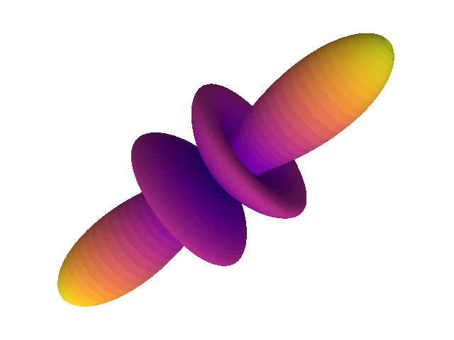
Using atom.scattering_rate, we can calculate the photon scattering for the angle pairs
(θ, φ) to generate a 3D plot of the emission pattern.
n_theta, n_phi = 128, 256
theta = np.linspace(0., np.pi, n_theta)
phi = np.linspace(0., 2 * np.pi, n_phi)
theta, phi = np.meshgrid(theta, phi, indexing="ij")

r = atom.scattering_rate(rho[0, :, :, -1], theta=theta, phi=phi,
                         x_vec=None, axis=0)
r /= np.max(r)
r = r.reshape((n_theta, n_phi))

x = r * np.sin(theta) * np.cos(phi)
y = r * np.sin(theta) * np.sin(phi)
z = r * np.cos(theta)

fig, ax = plt.subplots(subplot_kw={"projection": "3d"})

cm = plt.get_cmap("plasma")
ax.plot_surface(x, y, z, facecolors=cm(r), rcount=128, ccount=256,
                linewidth=0, antialiased=False)

xyz_lim = 0.7
ax.set_xlim(-xyz_lim, xyz_lim)
ax.set_ylim(-xyz_lim, xyz_lim)
ax.set_zlim(-xyz_lim, xyz_lim)
ax.set_box_aspect((1., 1., 1.))
ax.set_axis_off()
plt.subplots_adjust(left=0., bottom=0., right=1., top=1.)
plt.show()